Comparison
Probability distribution
cmap = cmocean.cm.ice
def zero_fill_prob_dist(dict, N):
    pn = {x: 0 for x in range(N)}
    for k, v in dict.items():
        pn[k] = v
    return pn
t_to_plot = 2
fig, ax = plt.subplots(1,1, figsize=(4,3))

ax.plot(pn_dict_pgf[t_to_plot].keys(), pn_dict_pgf[t_to_plot].values(), label="PGF", color=cmap(0.86), lw=2, zorder=-1)

ax.scatter(
    zero_fill_prob_dist(pn_dict_sim[t_to_plot], N_pgf).keys(),
    zero_fill_prob_dist(pn_dict_sim[t_to_plot], N_pgf).values(),
    # pn_dict_sim[t_to_plot].keys(), pn_dict_sim[t_to_plot].values(),
    label="Simulation", s=10, color=cmap(0.4)
)

ax.set_title(f"t={t_to_plot}", loc='left')
ax.set_ylabel("Probability")
ax.set_xlabel("$I_t$")

ax.set_xlim(-1, 100+1)

# ax.set_xscale('log')
# ax.set_yscale('log')

ax.legend(loc='upper right', frameon=False)

fig.tight_layout()
# plt.savefig('fig/fig_name.pdf', bbox_inches='tight')
plt.close()
show_fig_svg(fig)

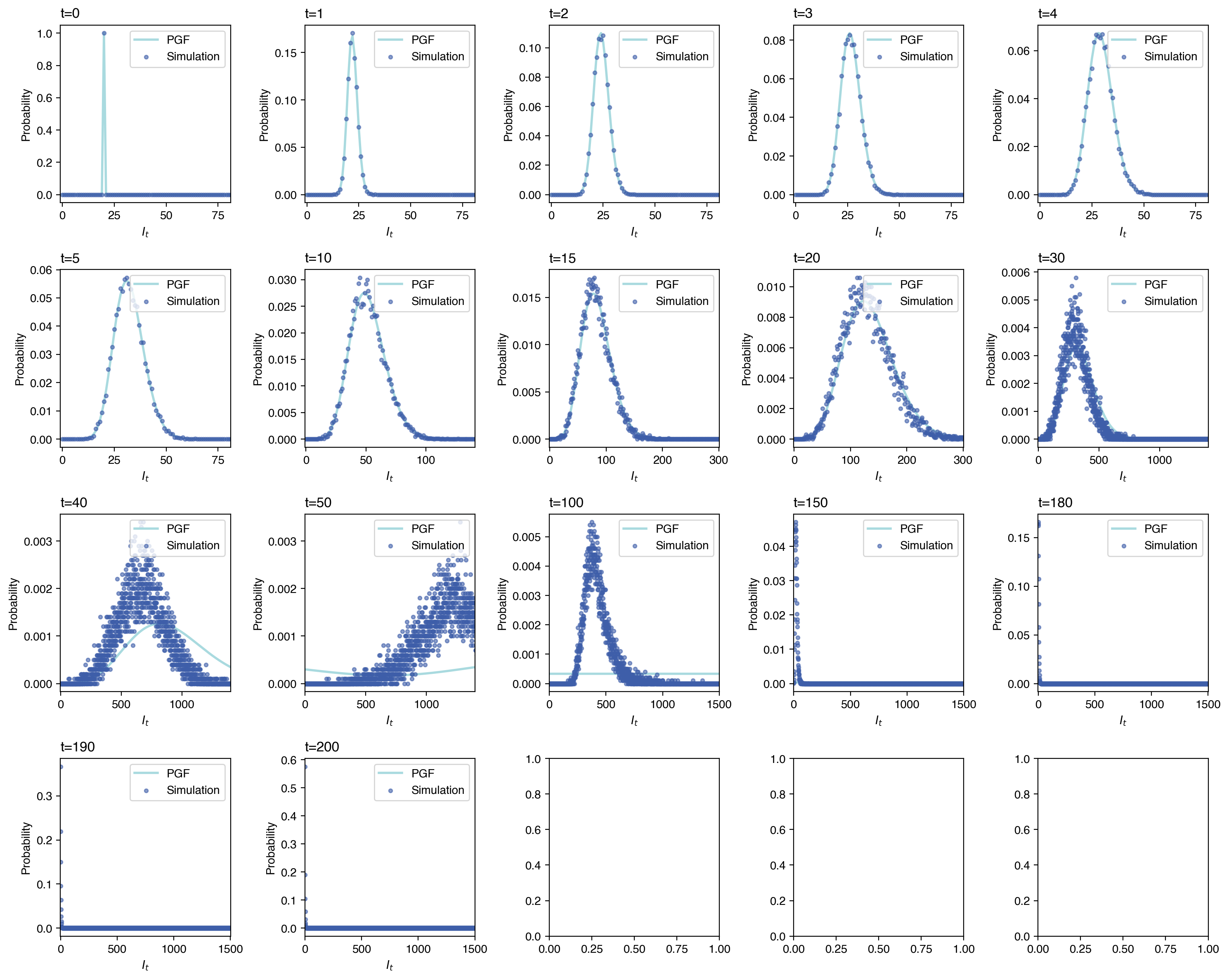
fig, axs = plt.subplots(4,5, figsize=(3*5,3*4))

axs_1d = axs.reshape(-1)

for i, t_ in enumerate([0,1,2,3,4,5,10,15,20,30,40,50,100,150,180,190,200]):
    ax = axs_1d[i]
    ax.plot(pn_dict_pgf[t_].keys(), pn_dict_pgf[t_].values(), label="PGF", color=cmap(0.86), lw=2, zorder=-1)

    ax.scatter(
        zero_fill_prob_dist(pn_dict_sim[t_], N_pgf).keys(),
        zero_fill_prob_dist(pn_dict_sim[t_], N_pgf).values(),
        label="Simulation", s=10, color=cmap(0.4),
        alpha=0.6
    )

    ax.set_title(f"t={t_}", loc='left')
    ax.set_ylabel("Probability")
    ax.set_xlabel("$I_t$")

    if t_ < 10:
        ax.set_xlim(-1, 80+1)
    elif t_ < 15:
        ax.set_xlim(-1, 140+1)
    elif t_ < 30:
        ax.set_xlim(-1, 300+1)
    elif t_ <= 50:
        ax.set_xlim(-1, 1400+1)
    else:
        ax.set_xlim(-1, 1500+1)

    # ax.set_xscale('log')
    # ax.set_yscale('log')

    ax.legend(loc='upper right', frameon=True)

fig.tight_layout()
    # plt.savefig('fig/fig_name.pdf', bbox_inches='tight')
plt.show()
estimates
# Compare mean I_t from stochastic determinations and the expected value of the distribution derived from  PGF
# We can see that the PGF esimation which uses Poisson approximation is only valid for t \lessapprox 100 in this case.
fig, ax = plt.subplots(1,1, figsize=(4,3))

ax.plot(It_summary.index, It_summary['mean'], label="Mean (Siml.)")
ax.fill_between(It_summary.index, It_summary['q25'], It_summary['q75'], alpha=0.2, label="IQR (Siml.)")

ax.plot(It_mean_pgf.keys(), It_mean_pgf.values(), label="Mean (PGF)")

ax.set_title("", loc='left')
ax.set_xlabel("Timestep")
ax.set_ylabel("$I_t$")

ax.legend(loc='center right', frameon=False)

fig.tight_layout()
# plt.savefig('fig/fig_name.pdf', bbox_inches='tight')
plt.close()
show_fig_svg(fig)

# Plot the difference between simulation and expected value from PGF method
fig, ax = plt.subplots(1,1, figsize=(4,3))

ax.plot(It_summary['mean'] - np.array(list(It_mean_pgf.values())))
ax.axhline(y=0, color='gray', linestyle='--', zorder=-1)

ax.set_title("", loc='left')

ax.set_xlabel("Timestep")
ax.set_ylabel(r"$\Delta$")

# ax.legend(loc='upper right', frameon=False)

fig.tight_layout()
# plt.savefig('fig/fig_name.pdf', bbox_inches='tight')
plt.close()
show_fig_svg(fig)

# This is because the Poisson approximation for Binomial distribution Bin(n,p) only holds when n is large and p is small.
# In this case, n and p corresponds to S_t and lambda.

fig, axs = plt.subplots(3,1, figsize=(4,3*3))
axs_1d = axs.reshape(-1)

axs_1d[0].plot(S_summary['mean'])
axs_1d[0].set_title("", loc='left')
axs_1d[0].set_xlabel("")
axs_1d[0].set_ylabel("$S_t$")

axs_1d[1].plot(lambda_summary['mean'])
axs_1d[1].set_title("", loc='left')
# axs_1d[1].set_xlabel("Timestep")
axs_1d[1].set_ylabel(r"$\lambda$")

axs_1d[2].plot(S_summary['mean'] * lambda_summary['mean'])
axs_1d[2].set_title("", loc='left')
axs_1d[2].set_xlabel("Timestep")
axs_1d[2].set_ylabel(r"$S_t \lambda$")

fig.tight_layout()
# plt.savefig('fig/fig_name.pdf', bbox_inches='tight')
plt.close()
show_fig_svg(fig)

Jensen-Shannon divergence of distributions
from scipy.spatial.distance import jensenshannon as js_distance
js_distance_dict = {}
for t_ in trange(n_steps):
    N_simmax = max(pn_dict_sim[t_].keys())+1
    zerofillmax = max(N_pgf, N_simmax)
    js_distance_dict[t_] = js_distance(
        list(zero_fill_prob_dist(pn_dict_pgf[t_], zerofillmax).values()),
        list(zero_fill_prob_dist(pn_dict_sim[t_], zerofillmax).values())
    )
100%|██████████| 200/200 [00:00<00:00, 1350.73it/s]fig, ax = plt.subplots(1,1, figsize=(4,3))
ax.plot(
js_distance_dict.keys(),
js_distance_dict.values()
)
ax.set_title("Jensen-Shannon Divergence", loc='left')
ax.set_xlabel("Timestep")
ax.set_ylabel("Distance")
# ax.set_xlim(-1,50)
fig.tight_layout()
# plt.savefig('fig/fig_name.pdf', bbox_inches='tight')
plt.close()
show_fig_svg(fig)
